Identifying, labelling, and plotting family relations from graphs

library(LTFHPlus)
library(dplyr)
library(igraph)

Introduction

This vignette demonstrates how to identify, label, and plot the total and/or average number of family relations per proband from graphs using the LTFHPlus package in R. We will use the minnbreast data set included in the kinship2 or Pedixplorer packages as example data. See documentation in one of those packages for details on the minnbreast data.

# load minnbreast data
data("minnbreast", package = "kinship2")
#printing a viewable version of the tibble:
rmarkdown::paged_table(minnbreast)

The minnbreast data has several columns, but the important ones for this application is the columns id, motherid, and fatherid, which contains the individual IDs and their parents’ IDs, respectively. The column proband indicates which individuals are probands (1 = proband, 0 = non-proband) in the minnbreast data. We will use this information later to only get family relations for the probands. We will create a graph with all individuals in the data and their familial links. We will refer to this graph as a population graph, as it contains all individuals in the population considered.

# create a (population) graph, with all individuals and all familial links
pop_graph = prepare_graph(.tbl = select(minnbreast, id, motherid, fatherid),
                          icol = "id",
                          fcol = "fatherid",
                          mcol = "motherid")

The population graph adds dummy links between siblings for kinship calculations. Removing these links means it is possible to read the number of individuals in the data and the number of identified familial links.

delete_edges(pop_graph, E(pop_graph)[which_mutual(pop_graph)])

## IGRAPH 0e473e0 DN-- 28081 30720 -- 
## + attr: name (v/c)
## + edges from 0e473e0 (vertex names):
##  [1] 25->3  4 ->3  1 ->4  2 ->4  1 ->5  2 ->5  1 ->6  2 ->6  1 ->7  2 ->7 
## [11] 1 ->8  2 ->8  1 ->9  2 ->9  1 ->10 2 ->10 5 ->11 26->11 5 ->12 26->12
## [21] 5 ->13 26->13 6 ->14 27->14 6 ->15 27->15 6 ->16 27->16 28->17 8 ->17
## [31] 29->18 9 ->18 29->19 9 ->19 29->20 9 ->20 24->21 3 ->21 24->22 3 ->22
## [41] 24->23 3 ->23 70->46 54->46 70->47 54->47 70->48 54->48 70->49 54->49
## [51] 70->50 54->50 70->51 54->51 70->52 54->52 70->53 54->53 44->54 45->54
## [61] 46->55 65->55 46->56 65->56 46->57 65->57 48->58 66->58 48->59 66->59
## [71] 48->60 66->60 67->61 50->61 79->62 53->62 69->63 53->63 69->64 53->64
## + ... omitted several edges

The minnbreast data has 28081 individuals and 30720 familial links.

The population graph can now be used to extract family graphs centred on a set of probands. The function get_family_graphs() allows us to specify a vector of proband IDs and the degree of relatives we want to include in the family graphs. The function get_family_graphs() also formats the data into a tibble with the columns fid and fam_graph (default names). The values in the column fid are the proband IDs, and the values in the column fam_graph are the corresponding neighbourhood graphs of the specified degree centred on each proband. These graphs are referred to as family graphs and are stored as igraph objects. Here, we will extract family graphs for all probands in the minnbreast data, including up to 10th degree relatives to ensure we capture all possible family members in the data.

# get family graphs for all probands in minnbreast data
family_graphs = get_family_graphs(pop_graph = pop_graph,
                                  ndegree = 10, # picking 10th degree relatives, to ensure we get all possible family members in the data
                                  proband_vec = as.character(minnbreast$id))
family_graphs

## # A tibble: 28,081 × 2
##    fid   fam_graph
##    <chr> <list>   
##  1 1     <igraph> 
##  2 2     <igraph> 
##  3 3     <igraph> 
##  4 4     <igraph> 
##  5 5     <igraph> 
##  6 6     <igraph> 
##  7 7     <igraph> 
##  8 8     <igraph> 
##  9 9     <igraph> 
## 10 10    <igraph> 
## # ℹ 28,071 more rows

We extract all probands next and identify and label their family relations using the get_relations() function. The function takes as input the family graphs and a vector of proband IDs. The output is a tibble with the columns fid, id1, id2, gen.x, gen.y, k, and lab. In order, they refer to the family the relation originiates from, the target indivial, the individual the label refers to, generations up, generations down, kinship, and label. In other words, id2’s relation to id1 is specified in the label column, lab, with additional information such as kinship and generational steps. The generational steps are used for plotting later.

# extracting just the set of individuals labelled as "proband" in the minnbreast data
proband_ids = minnbreast %>% filter(proband == 1) %>%
  pull(id)

labelled_data = get_relations(family_graphs = family_graphs, family_id_vec = proband_ids)
labelled_data

## # A tibble: 989,269 × 7
##    fid   id1   id2   gen.x gen.y     k lab  
##    <chr> <chr> <chr> <dbl> <dbl> <dbl> <chr>
##  1 4     1     3         0     2 0.125 GCh  
##  2 4     1     4         0     1 0.25  Ch   
##  3 4     1     5         0     1 0.25  Ch   
##  4 4     1     6         0     1 0.25  Ch   
##  5 4     1     7         0     1 0.25  Ch   
##  6 4     1     8         0     1 0.25  Ch   
##  7 4     1     9         0     1 0.25  Ch   
##  8 4     1     10        0     1 0.25  Ch   
##  9 4     1     11        0     2 0.125 GCh  
## 10 4     1     12        0     2 0.125 GCh  
## # ℹ 989,259 more rows

The labels are short-hand notation for familial relations. A list of the labels and what they mean can be seen here:

P: Proband
S: Sibling
GP: grandparents
2GP: great-grandparents (and 3GP for great-great-grandparents, etc.)
Ch: Child
GCh: Grandchild (and 2GCh for great-grandchild, etc.)
Pib: “Pibling” (parental sibling; aunt/uncle)
GPib: GrandPibling (grandparent’s sibling; 2GPib for great-grandparent’s sibling, etc.)
Nib: “Nibling” (sibling’s child; niece/nephew)
GNib: grandNibling (sibling’s grandchild; grand-niece/grand-nephew, etc.)
1C: First cousin
2C: Second cousin (and 3C for third cousin, etc.)
1C1R: First cousin once removed (and 2C1R for second cousin once removed, etc.)
1C2R: First cousin twice removed (and 2C2R for second cousin twice removed, etc.)
H-prefix: Half-relations, e.g. HS for half-sibling, H1C for half-first cousin, etc.

p2 = Relation_per_proband_plot(labelled_relations = labelled_data, proband_vec = proband_ids)
p2 # can be modified with ggplot2 functions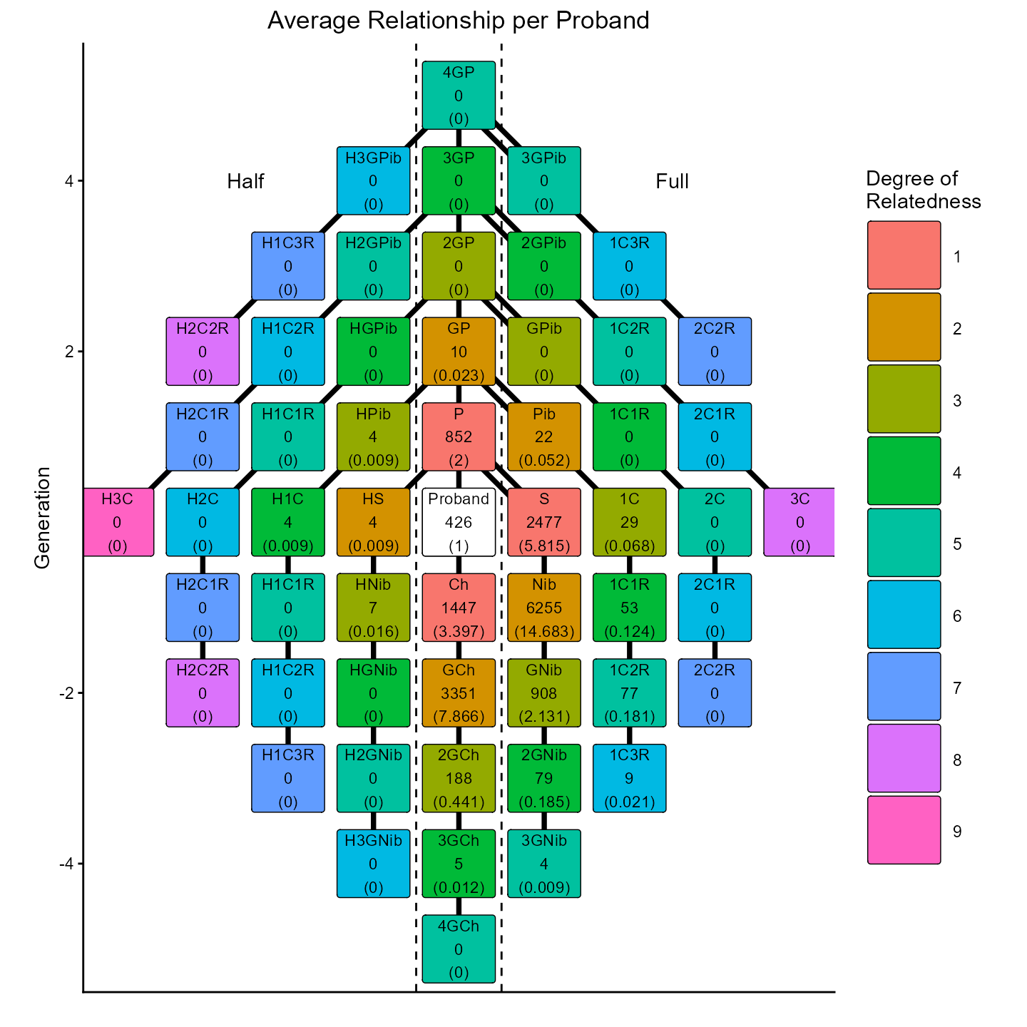

Plot of the identified relations per proband.

The function Relation_per_proband_plot() creates takes the labels in labelled_data and creates a plot with information from each proband specified in proband_vec by restricting to only the observations where these individuals appear in the id1 column. The default labels for each relation prints the label, the total number observed, and the average number observed. Alternatively, the report_label argument can be used to report only the total or only the average. The plot can be modified using ggplot2 functions as needed.

Emil Pedersen

2025-11-17

Introduction