From trio information to full families

Emil M. Pedersen

2025-11-17

library(LTFHPlus)
library(dplyr)
library(igraph)
library(kinship2)

In this document, we will present how we can go from trio information to full families that can be used to calculate kinship matrices. By trio information, we specifically mean knowing the id of the child and the id of the child’s mother and father. Kinship matrices are essential when estimating the liabilities with the estimate_liability() function of the package. This addition help with the process of identifying related individuals and subsequent construction of the kinship matrix.

From trio information to graph

The trio information can be used to create extended families manually by first identifying parents, grandparents, great-grandparents, etc.. From there, siblings, aunts and uncles, cousins, etc.. can also be identified. However, this is a tedious process and it is easy to miss family members. We have developed a function that can find all family member that are related of degree $n$ or closer that does not rely on the tedious process of identifying each family role manually.

Below is an example data set of a family. It contains half-siblings, half-aunts and -uncles, as well as cousins and individuals that have married into the family. An example is mgm meaning maternal grandmother, hspaunt meaning paternal half-aunt, or hsmuncleW meaning maternal half-uncle’s wife. We construct the example dataset with tribble because it enables row-wise construction, which mirrors how trio information is typically stored and helps readability in small example datasets.

# Setting seed:
set.seed(555)

# constructing family (trio) data
family = tribble(
  ~id, ~momcol, ~dadcol,
  "pid", "mom", "dad",
  "sib", "mom", "dad",
  "mhs", "mom", "dad2",
  "phs", "mom2", "dad",
  "mom", "mgm", "mgf",
  "dad", "pgm", "pgf",
  "dad2", "pgm2", "pgf2",
  "paunt", "pgm", "pgf",
  "pacousin", "paunt", "pauntH",
  "hspaunt", "pgm", "newpgf",
  "hspacousin", "hspaunt", "hspauntH",
  "puncle", "pgm", "pgf",
  "pucousin", "puncleW", "puncle",
  "maunt", "mgm", "mgf",
  "macousin", "maunt", "mauntH",
  "hsmuncle", "newmgm", "mgf",
  "hsmucousin", "hsmuncleW", "hsmuncle"
)

# simulating sex status on ambiguous individuals
thrs =  tibble(
 id = family %>% select(1:3) %>% unlist() %>% unique(),
 sex = case_when(
   id %in% family$momcol ~ "F",
   id %in% family$dadcol ~ "M",
   TRUE ~ NA)) %>% 
  mutate(sex = sapply(sex, function(x) ifelse(is.na(x), sample(c("M", "F"), 1), x)))

The object family is meant to represent the trio information that can be found in registers. It is possible to have multiple families in the same input data or single individuals with no family links.

graph = prepare_graph(.tbl = family, 
                      node_attributes = thrs,
                      fcol = "dadcol",
                      mcol = "momcol",
                      icol = "id")
graph

## IGRAPH 08de485 DN-- 31 44 -- 
## + attr: name (v/c), sex (v/c)
## + edges from 08de485 (vertex names):
##  [1] dad     ->pid        mom     ->pid        dad     ->sib       
##  [4] mom     ->sib        dad2    ->mhs        mom     ->mhs       
##  [7] dad     ->phs        mom2    ->phs        mgf     ->mom       
## [10] mgm     ->mom        pgf     ->dad        pgm     ->dad       
## [13] pgf2    ->dad2       pgm2    ->dad2       pgf     ->paunt     
## [16] pgm     ->paunt      pauntH  ->pacousin   paunt   ->pacousin  
## [19] newpgf  ->hspaunt    pgm     ->hspaunt    hspauntH->hspacousin
## [22] hspaunt ->hspacousin pgf     ->puncle     pgm     ->puncle    
## + ... omitted several edges

The object graph is a directed graph constructed from the trio information in family and is build using the igraph package. The direction in the graph is from parent to offspring.

From graph to subgraph and kinship matrix

We can construct a kinship matrix from all family members present in family, or we can consider only the family members that are of degree $n$. We can identify the family members of degree $2$ like this:

# get_family_graphs wraps make_ego_graph returns a formatted tbl
fam_graph = get_family_graphs(pop_graph = graph,
                              ndegree = 2,
                              proband_vec = V(graph)$name)
fam_graph

## # A tibble: 31 × 2
##    fid      fam_graph
##    <chr>    <list>   
##  1 pid      <igraph> 
##  2 sib      <igraph> 
##  3 mhs      <igraph> 
##  4 phs      <igraph> 
##  5 mom      <igraph> 
##  6 dad      <igraph> 
##  7 dad2     <igraph> 
##  8 paunt    <igraph> 
##  9 pacousin <igraph> 
## 10 hspaunt  <igraph> 
## # ℹ 21 more rows

fam_graph is a tibble with one row per proband (here all individuals in the graph are probands). The first column is the family ID, typically the name of the proband the family graph is centred around, and a column fam_graph containing the corresponding family graphs as igraph objects. We can plot one of the identified family graphs with the standard plot function from the igraph package, however it is not ideal for pedigrees past a certain size.

plot(fam_graph$fam_graph[[1]], # choosing pid's family graph 
     layout = layout_as_tree,
     vertex.size = 27.5,
     vertex.shape = "rectangle",
     vertex.label.cex = .75,
     edge.arrow.size = .3)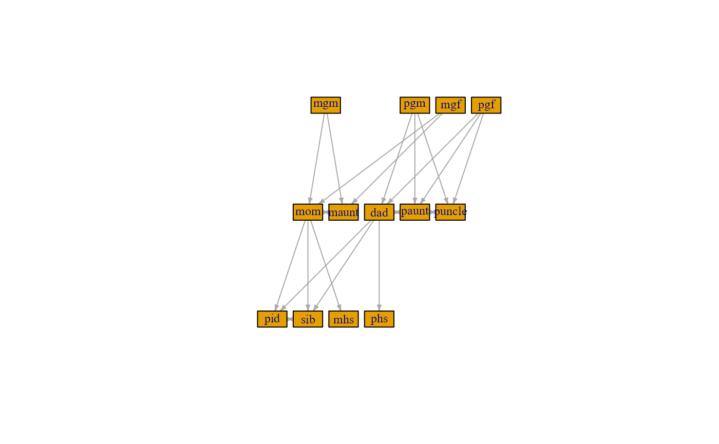 

In particular, individuals such as paternal uncle’s child (i.e a cousin, coded as pucousin above) is not present with this relatedness cut-off as such family members are of degree $3$.

Calculate kinship matrix

Finally, the kinship matrix can be calculated with get_kinship() in the following way:

get_kinship(fam_graph$fam_graph[[1]], h2 = 1, index_id = "pid", add_ind = FALSE)

##         pid  sib  mhs  phs mom dad paunt puncle maunt  mgm  pgm  mgf  pgf
## pid    1.00 0.50 0.25 0.25 0.5 0.5  0.25   0.25  0.25 0.25 0.25 0.25 0.25
## sib    0.50 1.00 0.25 0.25 0.5 0.5  0.25   0.25  0.25 0.25 0.25 0.25 0.25
## mhs    0.25 0.25 1.00 0.00 0.5 0.0  0.00   0.00  0.25 0.25 0.00 0.25 0.00
## phs    0.25 0.25 0.00 1.00 0.0 0.5  0.25   0.25  0.00 0.00 0.25 0.00 0.25
## mom    0.50 0.50 0.50 0.00 1.0 0.0  0.00   0.00  0.50 0.50 0.00 0.50 0.00
## dad    0.50 0.50 0.00 0.50 0.0 1.0  0.50   0.50  0.00 0.00 0.50 0.00 0.50
## paunt  0.25 0.25 0.00 0.25 0.0 0.5  1.00   0.50  0.00 0.00 0.50 0.00 0.50
## puncle 0.25 0.25 0.00 0.25 0.0 0.5  0.50   1.00  0.00 0.00 0.50 0.00 0.50
## maunt  0.25 0.25 0.25 0.00 0.5 0.0  0.00   0.00  1.00 0.50 0.00 0.50 0.00
## mgm    0.25 0.25 0.25 0.00 0.5 0.0  0.00   0.00  0.50 1.00 0.00 0.00 0.00
## pgm    0.25 0.25 0.00 0.25 0.0 0.5  0.50   0.50  0.00 0.00 1.00 0.00 0.00
## mgf    0.25 0.25 0.25 0.00 0.5 0.0  0.00   0.00  0.50 0.00 0.00 1.00 0.00
## pgf    0.25 0.25 0.00 0.25 0.0 0.5  0.50   0.50  0.00 0.00 0.00 0.00 1.00

A function called graph_to_trio() has been included in the package, which can convert from the graph object back into a trio object. This function is useful if you want to use the functionality of other packages that rely on trio information. One such example is using the plotting functionality of pedigrees in kinship2.

trio = graph_to_trio(graph = fam_graph$fam_graph[[1]], fixParents = TRUE)
trio

## # A tibble: 15 × 4
##    id      momid     dadid     sex  
##    <chr>   <chr>     <chr>     <chr>
##  1 pid     "mom"     "dad"     F    
##  2 sib     "mom"     "dad"     M    
##  3 mhs     "mom"     "added_2" F    
##  4 phs     "added_1" "dad"     F    
##  5 mom     "mgm"     "mgf"     F    
##  6 maunt   "mgm"     "mgf"     F    
##  7 dad     "pgm"     "pgf"     M    
##  8 paunt   "pgm"     "pgf"     F    
##  9 puncle  "pgm"     "pgf"     M    
## 10 mgf     ""        ""        M    
## 11 pgf     ""        ""        M    
## 12 mgm     ""        ""        F    
## 13 pgm     ""        ""        F    
## 14 added_1 ""        ""        F    
## 15 added_2 ""        ""        M

which can be used to utilise the powerful plotting tool kit available in the kinship2 package.

pedigree = with(trio,kinship2::pedigree(id = id, dadid = dadid,momid =  momid,sex =  sex))

plot(pedigree)